Classic VRPs¶

This notebook shows how to use PyVRP to solve two classic variants of the VRP: the capacitated vehicle routing problem (CVRP), and the vehicle routing problem with time windows (VRPTW). It builds on the tutorial by solving much larger instances, and going into more detail about the various plotting tools and diagnostics available in PyVRP.

A CVRP instance is defined on a complete graph \(G=(V,A)\), where \(V\) is the vertex set and \(A\) is the arc set. The vertex set \(V\) is partitioned into \(V=\{0\} \cup V_c\), where \(0\) represents the depot and \(V_c=\{1, \dots, n\}\) denotes the set of \(n\) customers. Each arc \((i, j) \in A\) has a weight \(d_{ij} \ge 0\) that represents the travel distance from \(i \in V\) to \(j \in V\). Each customer \(i \in V_c\) has a demand \(q_{i} \ge 0\). The objective is to find a feasible solution that minimises the total distance.

A VRPTW instance additionally incorporates time aspects into the problem. For the sake of exposition we assume the travel duration \(t_{ij} \ge 0\) is equal to the travel distance \(d_{ij}\) in this notebook. Each customer \(i \in V_c\) has a service time \(s_{i} \ge 0\) and a (hard) time window \(\left[e_i, l_i\right]\) that denotes the earliest and latest time that service can start. A vehicle is allowed to arrive at a customer location before the beginning of the time window, but it must wait for the window to open to start the delivery. Each vehicle must return to the depot before the end of the depot time window \(H\). The objective is to find a feasible solution that minimises the total distance.

Let’s first import what we will use in this notebook.

[1]:

import matplotlib.pyplot as plt
from tabulate import tabulate
from vrplib import read_solution

from pyvrp import Model, read
from pyvrp.plotting import (
    plot_coordinates,
    plot_instance,
    plot_result,
    plot_route_schedule,
)
from pyvrp.stop import MaxIterations, MaxRuntime

The capacitated VRP¶

Reading the instance¶

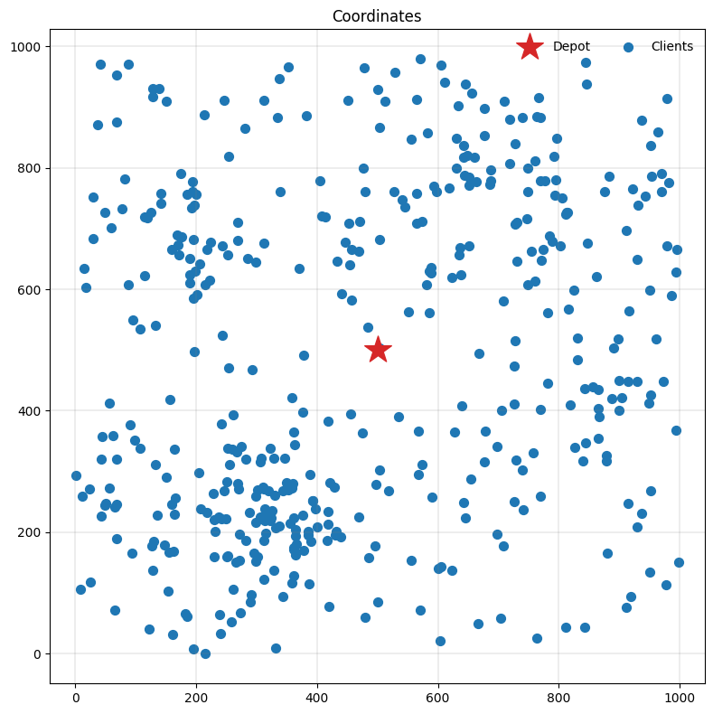
We will solve the X-n439-k37 instance, which is part of the X instance set that is widely used to benchmark CVRP algorithms. The function pyvrp.read reads the instance file and converts it to a ProblemData instance. We pass the argument round_func="round" to compute the Euclidean distances rounded to the nearest integral, which is the convention for the X benchmark set. We also load the best known solution to evaluate our solver later on.

[2]:

INSTANCE = read("data/X-n439-k37.vrp", round_func="round")
BKS = read_solution("data/X-n439-k37.sol")

Let’s plot the instance and see what we have.

[3]:

_, ax = plt.subplots(figsize=(8, 8))
plot_coordinates(INSTANCE, ax=ax)
plt.tight_layout()

Solving the instance¶

We will again use the Model interface to solve the instance. The Model interface supports a convenient from_data method that can be used to instantiate a model from a known ProblemData object.

[4]:

model = Model.from_data(INSTANCE)
result = model.solve(stop=MaxIterations(2000), seed=42, display=False)
print(result)

Solution results
================
    # routes: 37
   # clients: 438
   objective: 36977.00
# iterations: 2000
    run-time: 84.46 seconds

Routes
------
Route #1: 105 2 434 8 311 133 425 223 349 370 169 3
Route #2: 348 411 410 97 400 267 386 299 392 57 218 72
Route #3: 172 202 308 270 406 155 41 275 92 260 26 326
Route #4: 71 335 42 239 281 375 296 43 347 211 250 280
Route #5: 404 228 346 162 435 166 345 385 438 312 381 195
Route #6: 421 416 407 366 122 145 200 139 206 418 409 110
Route #7: 413 420 396 423 391 337 433 242 342 377 380 115
Route #8: 372 264 352 315 86 225 388 303 245 241 360 221
Route #9: 324 229 268 227 249 325 393 237 121 353 422 149
Route #10: 402 428 403 384 17 412 89 293 83 339 66 126
Route #11: 246 138 257 253 289 271 338 329 319 266 351 432
Route #12: 137 98 341 47 286 350 376 383 321 243 233 44
Route #13: 65 159 15 153 215 193 285 101 252 297 309 323
Route #14: 204 176 131 6 1 397 387 134 426 5 31 333
Route #15: 25 431 154 91 118 173 344 7 197 61 189 79
Route #16: 437 283 251 144 334 146
Route #17: 207 58 161 287 395 184 390 371 109 90 62 367
Route #18: 28 430 248 19 330 108 340 327 389 343 24 401
Route #19: 361 331 220 240 408 302 255 152 177 135 157 73
Route #20: 165 265 313 30 259 364 399 106 216 77 99 124
Route #21: 175 132 4 34 230 67 16 112 378 21 181 84
Route #22: 244 11 209 354 74 63 117 103 13 292 192 235
Route #23: 382 174 160 291 178 222 125 190 356 290 368 417
Route #24: 213 328 272 123 64 10 37 301 379 394 171 310
Route #25: 424 300 363 357 214 198 52 95 168 405 234 284
Route #26: 170 150 282 224 273 320 279 114 316 120 269 332
Route #27: 179 96 256 78 182 183 205 219 142 199 151 163
Route #28: 188 369 336 419 304 322 374 208 141 35 232 39
Route #29: 180 107 306 314 148 69 68 111 20 128 53 81
Route #30: 186 164 51 100 27 54 94 212 46 49 45 277
Route #31: 85 167 247 40 201 261 262 307 18 50 194 38
Route #32: 258 70 129 191 158 29 87 102 127 119 76 203
Route #33: 263 55 288 298 226 317 398 415 427 156 12 48
Route #34: 36 373 436 14 93 23 185 294 318 33 278 276
Route #35: 254 9 355 429 365 359 295 358 231 236 217 414
Route #36: 238 32 82 147 104 60 143 305 362 187 136 59
Route #37: 130 80 88 210 22 56 75 196 116 113 274 140

[5]:

gap = 100 * (result.cost() - BKS["cost"]) / BKS["cost"]
print(f"Found a solution with cost: {result.cost()}.")
print(f"This is {gap:.1f}% worse than the best known", end=" ")
print(f"solution, which is {BKS['cost']}.")

Found a solution with cost: 36977.
This is 1.6% worse than the best known solution, which is 36391.

We’ve managed to find a very good solution quickly!

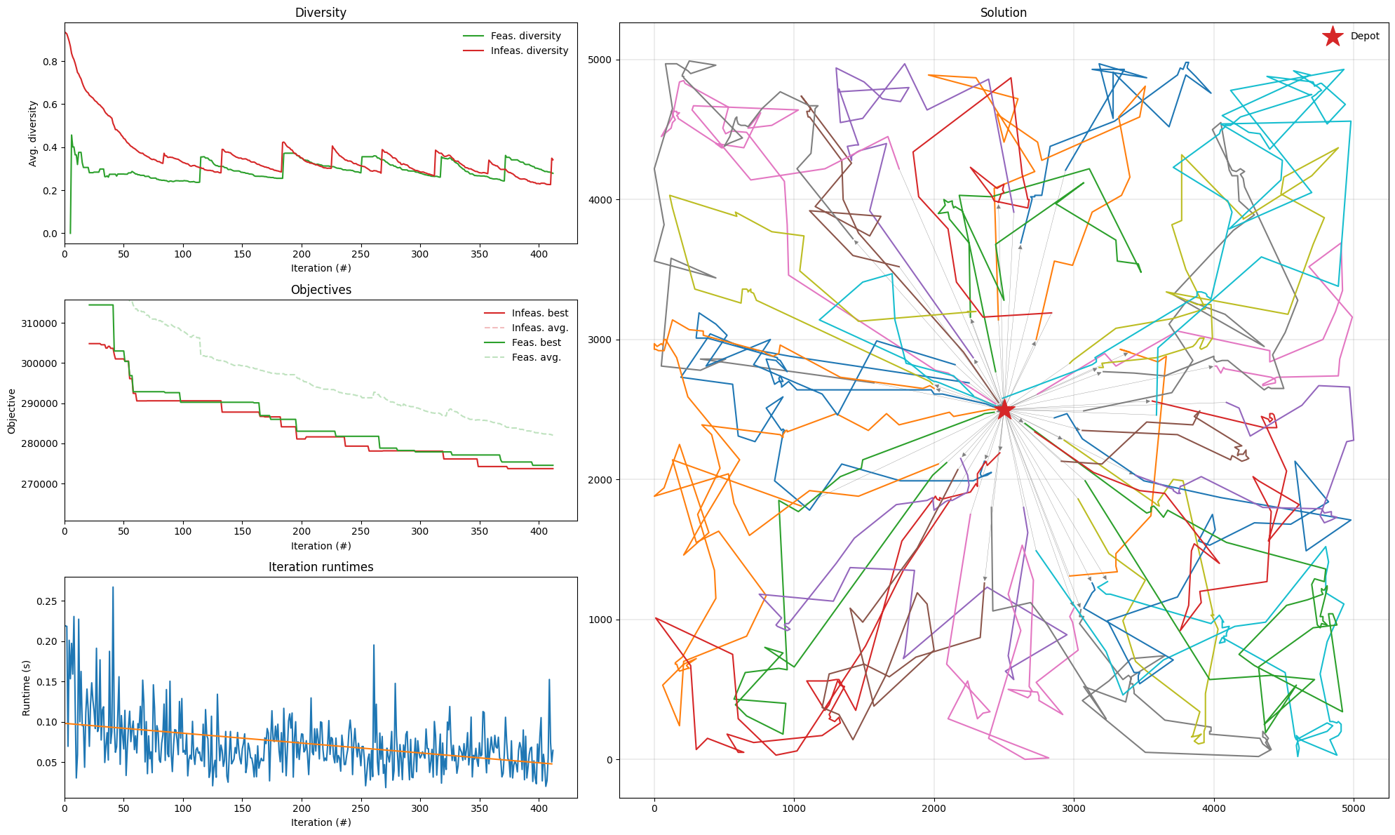
The Result object also contains useful statistics about the optimisation. We can now plot these statistics as well as the final solution use plot_result.

[6]:

fig = plt.figure(figsize=(15, 9))
plot_result(result, INSTANCE, fig)
fig.tight_layout()

PyVRP internally uses a genetic algorithm consisting of a population of feasible and infeasible solutions. These solutions are iteratively combined into new offspring solutions, that should result in increasingly better solutions. Of course, the solutions should not all be too similar: then there is little to gain from combining different solutions. The top-left Diversity plot tracks the average diversity of solutions in each of the feasible and infeasible solution populations. 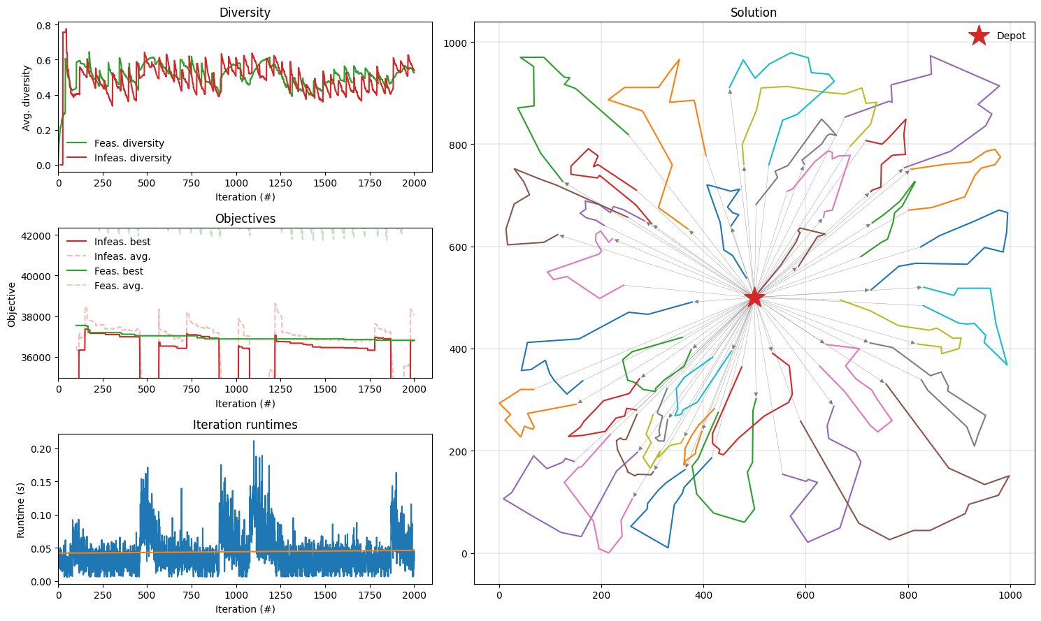The Objectives plot gives an overview of the best and average solution quality in the current population. The bottom-left figure shows iteration runtimes in seconds. Finally, the Solution plot shows the best observed solution.

The VRP with time windows¶

Reading the instance¶

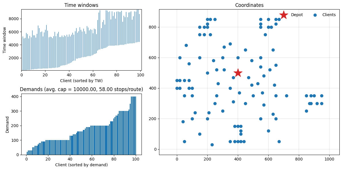
We start with a basic example that loads an instance and solves it using the standard configuration used by the Model interface. For the basic example we use one of the well-known Solomon instances.

We again use the function pyvrp.read. We pass the argument round_func="dimacs" following the DIMACS VRP challenge convention, this computes distances and durations truncated to one decimal place.

[7]:

INSTANCE = read("data/RC208.vrp", round_func="dimacs")
BKS = read_solution("data/RC208.sol")

Let’s plot the instance and see what we have. The function plot_instance will plot time windows, delivery demands and coordinates, which should give us a good impression of what the instance looks like. These plots can also be produced separately by calling the appropriate plot_* function: see the API documentation for details.

[8]:

fig = plt.figure(figsize=(12, 6))
plot_instance(INSTANCE, fig)

Solving the instance¶

We will again use the Model interface to solve the instance.

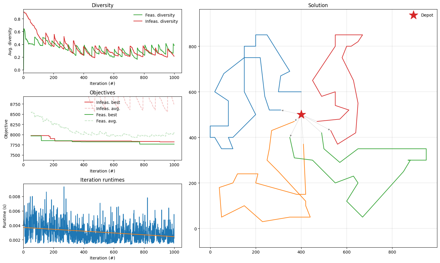
[9]:

model = Model.from_data(INSTANCE)
result = model.solve(stop=MaxIterations(1000), seed=42, display=False)
print(result)

Solution results
================
    # routes: 4
   # clients: 100
   objective: 7761.00
# iterations: 1000
    run-time: 2.50 seconds

Routes
------
Route #1: 90 65 82 99 52 83 64 49 19 18 48 21 23 25 77 58 75 97 59 87 74 86 57 24 22 20 66
Route #2: 94 92 95 67 62 50 34 31 29 27 26 28 30 32 33 76 89 63 85 51 84 56 91 80
Route #3: 61 42 44 39 38 36 35 37 40 43 41 72 71 93 96 54 81
Route #4: 69 98 88 2 6 7 79 73 78 12 14 47 17 16 15 13 9 11 10 53 60 8 46 4 45 5 3 1 70 100 55 68

[10]:

cost = result.cost() / 10
gap = 100 * (cost - BKS["cost"]) / BKS["cost"]
print(f"Found a solution with cost: {cost}.")
print(f"This is {gap:.1f}% worse than the optimal solution,", end=" ")
print(f"which is {BKS['cost']}.")

Found a solution with cost: 776.1.
This is 0.0% worse than the optimal solution, which is 776.1.

We’ve managed to find a (near) optimal solution in a few seconds!

[11]:

fig = plt.figure(figsize=(15, 9))
plot_result(result, INSTANCE, fig)
fig.tight_layout()

We can also inspect some statistics of the different routes, such as route distance, various durations, the number of stops and total delivery amount.

[12]:

solution = result.best
routes = solution.routes()

data = [
    {
        "num_stops": len(route),
        "distance": route.distance(),
        "service_duration": route.service_duration(),
        "wait_duration": route.wait_duration(),
        "time_warp": route.time_warp(),
        "delivery": route.delivery(),
    }
    for route in routes
]

header = list(data[0].keys())
rows = [datum.values() for datum in data]
tabulate(rows, header, tablefmt="html")

[12]:

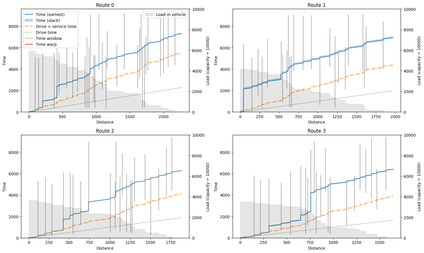
We can inspect the routes in more detail using the plot_route_schedule function. This will plot distance on the x-axis, and time on the y-axis, separating actual travel/driving time from waiting and service time. The clients visited are plotted as grey vertical bars indicating their time windows. We can see a jump to the start of the time window in the main (earliest) time line when a vehicle arrives early at a customer and has to wait. In some cases, there is slack in the route indicated by a semi-transparent region on top of the earliest time line. The grey background indicates the remaining load of the truck during the route, where the (right) y-axis ends at the vehicle capacity.

[13]:

fig, axarr = plt.subplots(2, 2, figsize=(15, 9))
for idx, (ax, route) in enumerate(zip(axarr.reshape(-1), routes)):
    plot_route_schedule(
        INSTANCE,
        route,
        title=f"Route {idx}",
        ax=ax,
        legend=idx == 0,
    )

fig.tight_layout()

Solving a larger VRPTW instance¶

To show that PyVRP can also handle much larger instances, we will solve one of the largest Gehring and Homberger VRPTW benchmark instances. The selected instance - RC2_10_5 - has 1000 clients.

[14]:

INSTANCE = read("data/RC2_10_5.vrp", round_func="dimacs")
BKS = read_solution("data/RC2_10_5.sol")

[15]:

fig = plt.figure(figsize=(15, 9))
plot_instance(INSTANCE, fig)

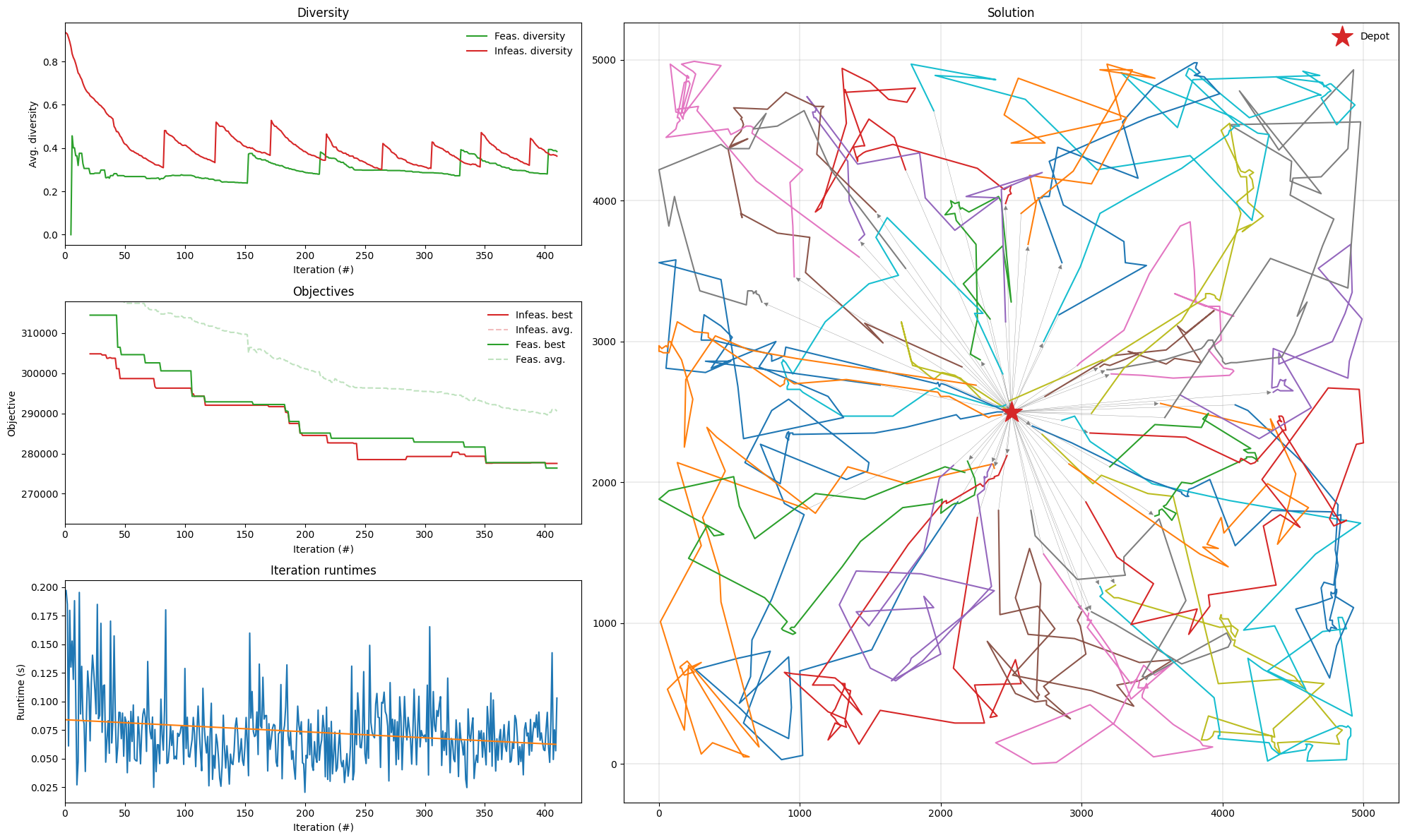
Here, we will use a runtime-based stopping criterion: we give the solver 30 seconds to compute.

[16]:

model = Model.from_data(INSTANCE)
result = model.solve(stop=MaxRuntime(30), seed=42, display=False)

[17]:

cost = result.cost() / 10
gap = 100 * (cost - BKS["cost"]) / BKS["cost"]
print(f"Found a solution with cost: {cost}.")
print(f"This is {gap:.1f}% worse than the best-known solution,", end=" ")
print(f"which is {BKS['cost']}.")

Found a solution with cost: 27570.2.
This is 6.9% worse than the best-known solution, which is 25797.5.

[18]:

plot_result(result, INSTANCE)
plt.tight_layout()

Conclusion¶

In this notebook, we used PyVRP’s Model interface to solve a CVRP instance with 438 clients to near-optimality, as well as several VRPTW instances, including a large 1000 client instance. Moreover, we demonstrated how to use the plotting tools to visualise the instance and statistics collected during the search procedure.