Using PyVRP’s components
We have relied on the Model interface to solve VRP instances in the examples so far. That high-level interface hides a lot of the components that available in PyVRP, which uses an iterated local search algorithm under the hood. In this notebook we will investigate these components in more detail to build our own solve function based on iterated local search.
Along the way we will solve the RC208.vrp instance, one of the well-known VRPTW benchmark instances of Solomon. This instance consists of 100 clients.
[1]:
from pyvrp import read

INSTANCE = read("data/RC208.vrp", round_func="dimacs")
We will implement a solve() function that will take a stop stopping criterion, and a seed for the random number generator. This definition is very close to that of Model.solve. The signature is
def solve(stop: StoppingCriterion, seed: int) -> Solution: ...
A tour of PyVRP
We need to understand the separate components in PyVRP before we are ready to implement this function. PyVRP uses an iterated local search algorithm under the hood. The IteratedLocalSearch object manages a current solution. In each iteration, the current solution is modified using a method from pyvrp.search – this method should perform both perturbation and improvement steps. This candidate solution is then considered for acceptance based on a dynamic threshold value. This process
continues until a stopping condition is reached (see pyvrp.stop for different conditions). Let’s have a look at the different parts of pyvrp that are used to implement this algorithm.
To instantiate the IteratedLocalSearch, we need to specify an initial solution, search method, penalty manager and random number generator. Let’s start with the random number generator because it is the easiest to set up.
Random number generator
[2]:
from pyvrp import RandomNumberGenerator

rng = RandomNumberGenerator(seed=42)
Search method
Let’s now define the search method. The search method applies both perturbation and improvement steps. PyVRP implements a LocalSearch method that is very customisable with different operators and search neighbourhoods. Different operators search different parts of the solution space, which can be beneficial in finding better solutions. The search neighbourhood defines which edges are evaluated. By restricting that set of edges the local search method works much faster.
We provide default operator sets and neighbourhoods, which can be used as follows.
[3]:
from pyvrp.search import NODE_OPERATORS, LocalSearch, compute_neighbours

neighbours = compute_neighbours(INSTANCE)
ls = LocalSearch(INSTANCE, rng, neighbours)

for node_op in NODE_OPERATORS:
    ls.add_node_operator(node_op(INSTANCE))
Solution representation and evaluation
We now have a functioning local search method. All we need are two additional components to make it work: an initial Solution containing a set of routes, and a CostEvaluator that can be used to evaluate different moves. Let’s define those.
[4]:
from pyvrp import CostEvaluator, Solution

sol = Solution.make_random(INSTANCE, rng)
cost_evaluator = CostEvaluator(
    load_penalties=[20],
    tw_penalty=20,
    dist_penalty=0,
)
The random solution sol that we created just yet is not feasible. This is not a problem, because PyVRP internally uses penalties to evaluate infeasibilities in each solution. This is done using the CostEvaluator’s penalised_cost function, which allows us to determine the quality of infeasible solutions as well.
[5]:
assert not sol.is_feasible()
print(cost_evaluator.penalised_cost(sol))
142556
Let’s see if the local search can improve this solution.
[6]:
new_sol = ls.search(sol, cost_evaluator)

assert not sol.is_feasible()
print(cost_evaluator.penalised_cost(new_sol))
8280
Much better! But the new solution is not yet feasible. Can we hammer out the infeasibilities by increasing the penalties?
[7]:
cost_evaluator = CostEvaluator([200], 200, 0)
new_sol = ls.search(sol, cost_evaluator)

assert new_sol.is_feasible()
How good is this solution?
[8]:
print(cost_evaluator.penalised_cost(new_sol))
8304
Pretty good! This is how PyVRP manages infeasibilities: it adjusts the penalty parameters to ensure sufficiently many solutions are feasible. Too few feasible solutions and the penalties go up; too many and they go down. This ensures a balanced search of feasible and infeasible solutions, which is good for exploration.
The object in charge of managing the penalty terms is the PenaltyManager, which can be asked to provide a CostEvaluator of the form we saw above.
[9]:
from pyvrp import PenaltyManager

pen_manager = PenaltyManager.init_from(INSTANCE)
cost_evaluator = pen_manager.cost_evaluator()
An initial solution can be constructed easily using the random solution constructor:
[10]:
init_sol = Solution.make_random(INSTANCE, rng)
We are now ready to construct the iterated local search algorithm.
[11]:
from pyvrp import IteratedLocalSearch

algo = IteratedLocalSearch(INSTANCE, pen_manager, rng, ls, init_sol)
We can call algo.run, which iterates until a stopping criterion is met. These stopping criteria can be imported from pyvrp.stop - see the API documentation for details.
[12]:
from pyvrp.stop import MaxIterations, MaxRuntime

iter_res = algo.run(stop=MaxIterations(2000))
time_res = algo.run(stop=MaxRuntime(1))  # seconds
Let’s investigate the solutions!
[13]:
print(iter_res)
Solution results
================
    # routes: 4
     # trips: 4
   # clients: 100
   objective: 7833
    distance: 7833
    duration: 17833
# iterations: 2000
    run-time: 1.28 seconds

Routes
------
Route #1: 90 65 82 99 52 83 64 49 19 18 48 21 23 25 77 58 75 97 59 87 74 86 57 24 22 20 66
Route #2: 61 81 94 93 71 72 42 44 43 40 36 35 37 38 39 41 54 96
Route #3: 92 95 67 62 50 34 31 29 27 26 28 30 32 33 76 89 63 85 51 84 56 91 80
Route #4: 69 98 88 2 6 79 73 78 12 14 47 16 17 15 13 9 11 10 53 60 7 8 46 4 45 5 3 1 70 100 55 68
[14]:
print(time_res)
Solution results
================
    # routes: 4
     # trips: 4
   # clients: 100
   objective: 7839
    distance: 7839
    duration: 17839
# iterations: 1578
    run-time: 1.00 seconds

Routes
------
Route #1: 92 95 67 62 50 34 31 29 27 26 28 30 32 33 76 89 63 85 51 84 56 91 80
Route #2: 90 65 82 99 52 83 64 49 19 18 48 21 23 25 77 58 75 97 59 87 74 86 57 24 22 20 66
Route #3: 69 98 88 53 78 12 14 47 16 15 13 9 10 11 17 73 79 7 2 8 46 45 5 3 1 4 6 60 55 100 70 68
Route #4: 61 81 94 93 71 72 42 44 43 40 36 35 37 38 39 41 54 96
The solve function
Let’s put everything we have learned together into a solve function.
[15]:
def solve(stop, seed):
    rng = RandomNumberGenerator(seed=seed)
    pm = PenaltyManager.init_from(INSTANCE)

    neighbours = compute_neighbours(INSTANCE)
    ls = LocalSearch(INSTANCE, rng, neighbours)

    for node_op in NODE_OPERATORS:
        ls.add_node_operator(node_op(INSTANCE))

    init = Solution.make_random(INSTANCE, rng)
    algo = IteratedLocalSearch(INSTANCE, pm, rng, ls, init)

    return algo.run(stop)
Very good. Let’s solve the instance again, now using the solve function.
[16]:
res = solve(stop=MaxIterations(2000), seed=1)
print(res)
Solution results
================
    # routes: 4
     # trips: 4
   # clients: 100
   objective: 7768
    distance: 7768
    duration: 17768
# iterations: 2000
    run-time: 1.28 seconds

Routes
------
Route #1: 69 98 88 2 6 7 79 73 78 12 14 47 17 16 15 13 9 11 10 53 60 8 46 4 45 5 3 1 70 100 55 68
Route #2: 90 65 82 99 52 83 64 49 19 18 48 21 23 25 77 58 75 97 59 87 74 86 57 24 22 20 66
Route #3: 81 61 42 44 39 38 36 35 37 40 43 41 72 71 93 94 96 54
Route #4: 92 95 67 62 50 34 31 29 27 26 28 30 32 33 76 89 63 85 51 84 56 91 80
PyVRP also provides many plotting tools that can be used to investigate a data instance or solution result.
[17]:
import matplotlib.pyplot as plt

from pyvrp.plotting import plot_result
[18]:
fig = plt.figure(figsize=(12, 8))

plot_result(res, INSTANCE, fig=fig)
plt.tight_layout()
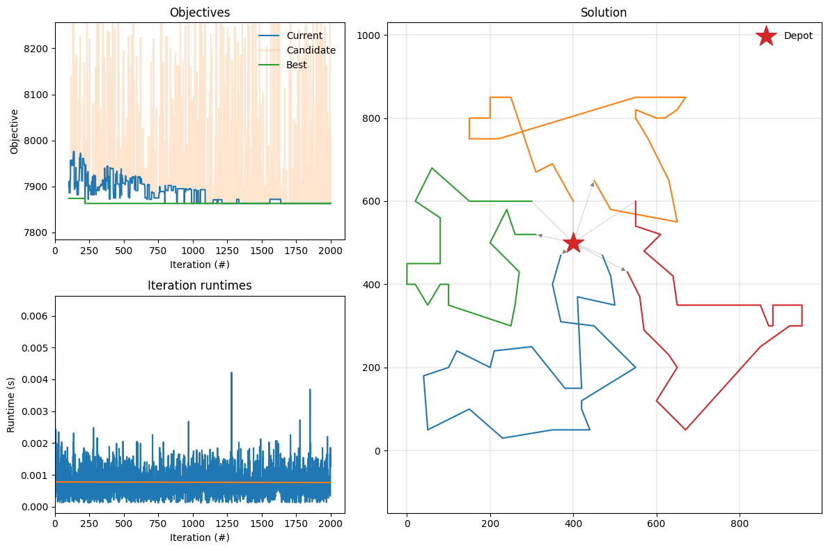
The top-left figure shows the penalised costs of the current, candidate, and best solutions across iterations. The fluctuations in current solution cost demonstrates the acceptance criterion’s strategy: while generally favoring improvements, it occasionally accepts worse solutions to escape local minima. Meanwhile, the candidate solution cost variations show the perturbation strategy - generating diverse solutions that, although occasionally being significantly worse, are essential to finding superior solutions throughout the search. The bottom-left figure shows average iteration runtimes (in seconds). Finally, the figure on the right plots the best observed solution.
Conclusion
In this notebook we have used some of the different components in PyVRP to implement our own solve function. Along the way we learned about how PyVRP works internally.